Analyzing the Mothur MiSeq SOP dataset with Phyloseq

By Dr. Thomas H.A. Haverkamp 3/14/2018

This is a tutorial on the usage of an r-packaged called Phyloseq. It is a large R-package that can help you explore and analyze your microbiome data through vizualizations and statistical testing. In this tutorial we will use the data produced in the Mothur MiSeq SOP. It is a small and simple dataset and excellent for teaching purposes. The Phyloseq package can handle much more complex datasets, but even with this limited dataset, we can experience the usefulness of Phyloseq. Phyloseq has a wide range of options and can analyze data produced from various sources such as mothur, qiime and from biome-formatted datasets. It can merge different datasets (data-types) into a single phyloseq object (more on that below). It comes with a variety of example datasets that can easily be accessed after loading the phyloseq package an all it’s dependencies.

This tutorial is written for use in the biolinux environment. However, if you are working in a different environment (e.g. Windows, Mac OSX, Linux), you can still follow this tutorial. Make sure your R-version is up to date. (minimum R-version that worked for me: 3.4.1)

The tutorial starts by first doing a little work in Mothur in order to make the tutorial a little more interesting, and show a functionality that is nice for exploring microbiome datasets.

The next step if for the biolinux. Phyloseq will not install properly on the biolinux version 8.0.7, since that has an old version of R (version 3.2.0). Thus, we need to upgrade R to the newest available version.

After the preperatory work, and after making sure that the right R version (version 3.4.1 or above) is working, we start setting up the R environment. That means installation of various R-packages including phyloseq.

Please send any comments / questions to my gmail.com address: Thhaverk

Acknowledgments.

This tutorial was created using the invaluable help of google and many interesting other tutorials, or even complete overviews of the R-code from specific publications. Without those sources I could not have made the current page. Below you find a few of the websites (many of them written in R-markdown) which I would like to point out, since they were excellent and inspired me to work out this tutorial. This tutorial was created for the bioinformatics course at the Norwegian veterinary institute.

A little mothur pre-work before the tutorial

The prework consists of making a tree from the OTU sequences found in the entire dataset. The reason for this is that with phyloseq we can vizualize which OTUs are found in the microbiome study samples, or the treatment, and identify if there closely related OTUs present in other samples or other treatments. This can be helpful for exploring how your samples relate to each other, and how widespread the OTUs are.

In order to create a tree, we will first need to extract representative sequences from each OTU before we can use that to create a distance matrix and then in the end a *.tre file with the dendrogram.

# mothur command to extract for each OTU a representative sequence
get.oturep(column=final.dist, list=final.list, fasta=final.fasta, count=final.count_table, label=0.03)

This creates a file with fasta sequences, but the headers are a bit problematic for usage in the phyloseq package. Run the below command in Mothur with the command: system

head -n 1 MiSeq_SOP/final.0.03.rep.fasta

>M00967_43_000000000-A3JHG_1_1101_13234_1983    Otu0001|12285|F3D0-F3D1-F3D141-F3D142-F3D143-F3D144-F3D145-F3D146-F3D147-F3D148-F3D149-F3D150-F3D2-F3D3-F3D5-F3D6-F3D7-F3D8-F3D9

The above head command shows that the fasta headers have the original fasta sequence name followed by the OTU label, the number of sequences in the complete dataset for that OTU, and all the samples where this OTU is found. That is all important data, but if we want to read it into phyloseq, there is a problem. Phyloseq expects to have the OTU label as the name of the sequence, and nothing else. So we have to modify the fasta headers of all sequences to only have the OTU-label. We will use two sed commands that we pipe ( “

” ) after each other so that we end up with the proper filenames. Run these again in mothur using the system command.

sed 's/>M.*Otu/>Otu/g' MiSeq_SOP/final.0.03.rep.fasta |sed -e 's/|.*//g'> MiSeq_SOP/final.0.03.rep.otu.fasta

head -n 1 MiSeq_SOP/final.0.03.rep.otu.fasta

>Otu0001

Now we can continue with the commands to create a dendrogram from the OTU sequences.

#calculate distances between the representative sequences
dist.seqs(fasta=final.0.03.rep.otu.fasta, output=lt, processors=32)

# use the distance file in the command clearcut to generate a neighbor-joining phylogeny of the OTU sequences
clearcut(phylip=final.0.03.rep.otu.phylip.dist)

The clearcut command used the distance matrix to produce the *.tre file, which contains a dendrogram showing the distance relation between all OTUs’. A program called treeview could do that in biolinux. However, the R-package phyloseq can also do that in R. I will show that, but before doing that we first we need to set-up R-studio.

Setting up R to work with the phyloseq package.

Phyloseq is a big R-package and it needs quite a few other R-packages in order to function appropriately. We therefor start with first checking which version of R we have, and then we will be installing all the required packages and get them up to date.

Checking the r version. BIOLINUX

Open R-studio and in the console type:

version

##                _                           
## platform       x86_64-apple-darwin15.6.0   
## arch           x86_64                      
## os             darwin15.6.0                
## system         x86_64, darwin15.6.0        
## status                                     
## major          3                           
## minor          4.1                         
## year           2017                        
## month          06                          
## day            30                          
## svn rev        72865                       
## language       R                           
## version.string R version 3.4.1 (2017-06-30)
## nickname       Single Candle

# or for only the version type
R.version.string

This shows that I am running R-version 3.4.1 and an x86_64-apple system. That is the version that worked for me. However, if you are running biolinux version 8.0.7 we first need to do a bit of updating of the R-system since that system is using an old version of R (version 3.2.0), which is not compatible with phyloseq. So close R-studio, and log-out of your user account on the biolinux system.

Installing a newer version of R on Biolinux

The task here is: first uninstall R to clean-up the environment, and then we need to install the latest version of R (currently 3.4.4) that is available for the Ubuntu version 14.04 lTS (“Trusty”). It is not easy but it is a necessary step, and without this, the whole tutorial can not be done within biolinux.

The manual

Please follow this as closely as possible!!!

Log into the biolinux machine as the system manager, and make sure the other users (You) are not active as well.
We first need to uninstall R program, before we can install a new one. Go to the application manager program (on the left side of your screen, a icon that looks like a bag with an “A”). When it is started use the search box to type “R “ (wit a space after the R). Then select uninstall. After this is finished restart the biolinux machine.
Restart the biolinux machine and make sure you log in as the system manager.
Open a terminal and type:
```
sudo nano /etc/apt/sources.list
```
This opens nano and because we use sudo it allows us to edit the sources.list file. The tool called apt, use this list to find the software it needs to update. We need to get a new R version and by adding the following line we enable apt to install an newer version of R on our biolinux system. So scroll to the last line of the file add an empty line and then add the following three lines:
```
## Adding the CRAN mirror from the University of Bergen, to 
## obtain the latest R version
deb https://cran.uib.no/bin/linux/ubuntu trusty/
```
After typing this, save the file and close nano. Now we have added a internet address where the the tool apt can find the latest version of R.
Next, do we use the tool apt to update the signature files needed for identifying where we can download R and all kinds of other software. In the terminal we now type:
```
sudo apt-get update
```
When this is finished we see a bunch or error messages. Those indicate that apt-get could not identify certain websites since signature keys were too old. Since we updated the sources.list file with a new website, we should not have this problem for the particular website we added to that file.
Next we are going to install R version 3.4.4, which is called: “Someone to Lean On”. R versions come with funky names.

After running the next command you will get three questions, you should answer them like this: “Yes”, “Yes”, “N”. The command to install R is:
```
sudo apt-get install r-base
```
When this is finished, type “R” on the commandline. That should start a new version of R in the terminal. Use “quit()” to stop R again.
Log out of the system manager account and log in to your own user account, and then start-up R-studio. Now we are ready to start with the phyloseq tutorial.

Installing of phyloseq and it’s dependencies.

Note, that we preferably want the latest versions.

Installing phyloseq and all the dependecies

We are installing the phyloseq version from the bioconductor website and we want to do that in such a way that it is installed in the root directory.

Start R-studio and opena blank “R script”. Start by writting these commands to install phyloseq in the R script. When asked to install in a personal library, say “NO”

#installing the phyloseq package
source('http://bioconductor.org/biocLite.R')
biocLite('phyloseq')

This takes quite some time, since phyloseq needs a lot of additional packages in order to function.

Now close Rstudio and then open it again. Somehow there is a bug which does not show the installed packages for this step.

```

After writting each command use **ctrl return* to run the commands.

Installing ggplot (an advanced graphic package) and its dependencies

Next we could install ggplot2, which is a R-package able to produce fancy graphs that can be tweaked in almost anyway we can think of. Here are examples of ggplot2 graphs together with code on how they were created. Feel free to try out the code yourself, the data needed is available in the scripts. Below are the commands for the installation of ggplot2, but phyloseq has installed that already. See in the packages list in Rstudio if ggplot2 is installed.

# installing ggplot2
install.packages("ggplot2", type="source")

Installing additional packages

Phyloseq relies heavily on extra packages for manipulation of datasets, manipulation of graphs. So we add to packages that are needed as well.

# installing additional packages
install.packages("dplyr") # data manipulation packages
install.packages("cowplot") # to combine multiple ggplot images into one figure

Now have we installed all the R-packages needed for this tutorial and we are ready to start with the actual data analysis.

Setting up the R environment for the analysis.

After installing all the packages needed for the phyloseq tutorial, we need to load them into the R environment using the command library.

# loading libraries
library(ggplot2)
library(vegan) # ecological diversity analysis
library(dplyr)
library(scales) # scale functions for vizualizations
library(grid)
library(reshape2) # data manipulation package
library(cowplot)
library(phyloseq)

The next step is to set-up our system. We direct R to use a specific working directory, where our data is stored. And we set-up a theme, which we can use to make our graphs pretty. Today we use a simple theme that makes that the graphs have a white background and black lines. For more on ggplot2 themes I recommend this tutorial.

# setting the working directory
setwd("~/Desktop/amplicons/")

# Set plotting theme
theme_set(theme_bw())

Importing the mothur MiSeq SOP data.

Phyloseq wants to have all data available for a microbiome dataset combined into one single object. So different microbiome datasets (mothur, qiime etc) needs to be imported in a specific way. Thus phyloseq comes with a range of import functions. Since we have data from mothur, we use the phyloseq command: import_mothur.

The mothur data we import, is the data after we have created the OTU tables (shared file) when following the MiSeq SOP. Remember that we created OTUs at the 97 % similarity cut-off, but other levels are also possible. See this recent publication on why the similarity cut-off might be stricter, or why you might want to use oligotypes to describe community differences.

# Assign variables for imported data
sharedfile = "MiSeq_SOP/final.shared"
taxfile = "MiSeq_SOP/final.0.03.taxonomy"
treefile <- "MiSeq_SOP/final.0.03.rep.otu.phylip.tre" 
mapfile = "MiSeq_SOP/mouse.dpw.metadata"

# Import mothur data
mothur_data <- import_mothur(mothur_shared_file = sharedfile,
                             mothur_constaxonomy_file = taxfile,
                             mothur_tree_file = treefile)

Note, that we are not adding the metadata to the phyloseq object ** mothur_data**. The sample metadata (mouse.dpw.metadata) is a tab delimited file that needs to be modified a little bit before we can add it to the object: mothur_data. We do that in the following way

# import samples metadata in R
map <- read.delim(mapfile)

If we check the metadata we find that it is in a normal tab delimited format, which phyloseq will not accept.

# checking the first few lines of the dataframe "map"
head(map)

##    group dpw
## 1   F3D0   0
## 2   F3D1   1
## 3 F3D141 141
## 4 F3D142 142
## 5 F3D143 143
## 6 F3D144 144

Next do we add two colums. the first column contains the factor “time” and the second column, contains FAKE data for bodyweights. We use this fake data for teaching how constrained ordinations can be used.

#modifying the dataframe "map"
map$time <- c("early", "early", rep("late", 10), rep("early", 7))

# Adding FAKE body weight data for pups post weaning and adults for use in constrained ordinations
# Note this data is only added for teaching purposes, and is completely unnatural, except the first weight.
# For the pups we use increasing body_weights.
# For the body weights of the late time points, I sample a normal distribution with a mean of 40, to make it random.
# it is important to set the seed, to make the results reproducible
set.seed(1)

# adding FAKE body weights
map$body_weight <- c(11, 12, 
                     round(rnorm(10, mean =40, sd = 1),digits=2),
                     seq (13, 30, by = 2.5)
                     )
#checking the dataframe "map"
str(map)

## 'data.frame':    19 obs. of  4 variables:
##  $ group      : Factor w/ 19 levels "F3D0","F3D1",..: 1 2 3 4 5 6 7 8 9 10 ...
##  $ dpw        : int  0 1 141 142 143 144 145 146 147 148 ...
##  $ time       : chr  "early" "early" "late" "late" ...
##  $ body_weight: num  11 12 39.4 40.2 39.2 ...

We are almost there with the modification of the metadata. The next step is to transfer the dataframe “map” in a phyloseq object called “map”. After that we need one more step before we merge the object “map” to the object “mothur_data”. The only formatting required to merge the metadata object “map” is that the rownames must match the sample names in your shared and taxonomy files.

# transform dataframe into phyloseq class object.
map <- sample_data(map)

# Assign rownames to be Sample ID's
rownames(map) <- map$group

#checking the object "map"
str(map)

## 'data.frame':    19 obs. of  4 variables:
## Formal class 'sample_data' [package "phyloseq"] with 4 slots
##   ..@ .Data    :List of 4
##   .. ..$ : Factor w/ 19 levels "F3D0","F3D1",..: 1 2 3 4 5 6 7 8 9 10 ...
##   .. ..$ : int  0 1 141 142 143 144 145 146 147 148 ...
##   .. ..$ : chr  "early" "early" "late" "late" ...
##   .. ..$ : num  11 12 39.4 40.2 39.2 ...
##   ..@ names    : chr  "group" "dpw" "time" "body_weight"
##   ..@ row.names: chr  "F3D0" "F3D1" "F3D141" "F3D142" ...
##   ..@ .S3Class : chr "data.frame"

The next step is that we merge the metadata file with the phyloseq formated file mothur_data.

# Merge mothurdata object with sample metadata
mothur_merge <- merge_phyloseq(mothur_data, map)

# showing the object mothur_merge
mothur_merge

## phyloseq-class experiment-level object
## otu_table()   OTU Table:         [ 394 taxa and 19 samples ]
## sample_data() Sample Data:       [ 19 samples by 4 sample variables ]
## tax_table()   Taxonomy Table:    [ 394 taxa by 6 taxonomic ranks ]
## phy_tree()    Phylogenetic Tree: [ 394 tips and 393 internal nodes ]

At this point have we create a phyloseq-class object called: “mothur_merge”. If we wanted to, we could add more data to this object. At anytime, we can print out the data structures stored in a phyloseq object to quickly view its contents. In addition, we also look at part of the dataset stored in this phyloseq object. Let’s try that.

# listing the first 10 lines of the taxonomy table
head(mothur_merge@tax_table, n=10)

## Taxonomy Table:     [10 taxa by 6 taxonomic ranks]:
##         Rank1      Rank2        Rank3        Rank4          
## Otu0099 "Bacteria" "Firmicutes" "Clostridia" "Clostridiales"
## Otu0025 "Bacteria" "Firmicutes" "Clostridia" "Clostridiales"
## Otu0151 "Bacteria" "Firmicutes" "Clostridia" "Clostridiales"
## Otu0100 "Bacteria" "Firmicutes" "Clostridia" "Clostridiales"
## Otu0124 "Bacteria" "Firmicutes" "Clostridia" "Clostridiales"
## Otu0080 "Bacteria" "Firmicutes" "Clostridia" "Clostridiales"
## Otu0208 "Bacteria" "Firmicutes" "Clostridia" "Clostridiales"
## Otu0102 "Bacteria" "Firmicutes" "Clostridia" "Clostridiales"
## Otu0199 "Bacteria" "Firmicutes" "Clostridia" "Clostridiales"
## Otu0130 "Bacteria" "Firmicutes" "Clostridia" "Clostridiales"
##         Rank5             Rank6                          
## Otu0099 "Lachnospiraceae" "Lachnospiraceae_unclassified" 
## Otu0025 "Lachnospiraceae" "Lachnospiraceae_unclassified" 
## Otu0151 "Lachnospiraceae" "Lachnospiraceae_unclassified" 
## Otu0100 "Lachnospiraceae" "Lachnospiraceae_unclassified" 
## Otu0124 "Lachnospiraceae" "Lachnospiraceae_unclassified" 
## Otu0080 "Lachnospiraceae" "Roseburia"                    
## Otu0208 "Lachnospiraceae" "Roseburia"                    
## Otu0102 "Lachnospiraceae" "Roseburia"                    
## Otu0199 "Lachnospiraceae" "Lachnospiracea_incertae_sedis"
## Otu0130 "Lachnospiraceae" "Dorea"

#OR in a slight different way:
head(tax_table(mothur_merge), n=10)

## Taxonomy Table:     [10 taxa by 6 taxonomic ranks]:
##         Rank1      Rank2        Rank3        Rank4          
## Otu0099 "Bacteria" "Firmicutes" "Clostridia" "Clostridiales"
## Otu0025 "Bacteria" "Firmicutes" "Clostridia" "Clostridiales"
## Otu0151 "Bacteria" "Firmicutes" "Clostridia" "Clostridiales"
## Otu0100 "Bacteria" "Firmicutes" "Clostridia" "Clostridiales"
## Otu0124 "Bacteria" "Firmicutes" "Clostridia" "Clostridiales"
## Otu0080 "Bacteria" "Firmicutes" "Clostridia" "Clostridiales"
## Otu0208 "Bacteria" "Firmicutes" "Clostridia" "Clostridiales"
## Otu0102 "Bacteria" "Firmicutes" "Clostridia" "Clostridiales"
## Otu0199 "Bacteria" "Firmicutes" "Clostridia" "Clostridiales"
## Otu0130 "Bacteria" "Firmicutes" "Clostridia" "Clostridiales"
##         Rank5             Rank6                          
## Otu0099 "Lachnospiraceae" "Lachnospiraceae_unclassified" 
## Otu0025 "Lachnospiraceae" "Lachnospiraceae_unclassified" 
## Otu0151 "Lachnospiraceae" "Lachnospiraceae_unclassified" 
## Otu0100 "Lachnospiraceae" "Lachnospiraceae_unclassified" 
## Otu0124 "Lachnospiraceae" "Lachnospiraceae_unclassified" 
## Otu0080 "Lachnospiraceae" "Roseburia"                    
## Otu0208 "Lachnospiraceae" "Roseburia"                    
## Otu0102 "Lachnospiraceae" "Roseburia"                    
## Otu0199 "Lachnospiraceae" "Lachnospiracea_incertae_sedis"
## Otu0130 "Lachnospiraceae" "Dorea"

We can see that the headers from the taxonomy table are not really nice. Rank 1, 2, 3 etc is not understandable, so we need to reformat the column names in the taxonomy table.

#renaming taxonomy column names
colnames(tax_table(mothur_merge)) <- c("Kingdom", "Phylum", "Class", 
  "Order", "Family", "Genus")

Checking them using the colnames command

colnames(tax_table(mothur_merge))

## [1] "Kingdom" "Phylum"  "Class"   "Order"   "Family"  "Genus"

Filtering out unwanted taxa from our analysis.

Now we will filter out Eukaryotes, Archaea, chloroplasts and mitochondria, because we only intended to amplify bacterial sequences. You may have done this filtering already in mothur, but it’s good to check you don’t have anything lurking in the taxonomy table. I like to keep these organisms in my dataset when running mothur because they are easy enough to remove with Phyloseq and sometimes I’m interested in exploring them. We will then create our final phyloseq object called: “mouse_data”.

# create object mouse_data
mouse_data <- mothur_merge %>%
  subset_taxa(
    Kingdom == "Bacteria" &
    Family  != "mitochondria" &
    Class   != "Chloroplast"
  )

#show mouse data
mouse_data

## phyloseq-class experiment-level object
## otu_table()   OTU Table:         [ 390 taxa and 19 samples ]
## sample_data() Sample Data:       [ 19 samples by 4 sample variables ]
## tax_table()   Taxonomy Table:    [ 390 taxa by 6 taxonomic ranks ]
## phy_tree()    Phylogenetic Tree: [ 390 tips and 389 internal nodes ]

This was quite a bit of work in order to just get to the start of our microbiome analysis.

Now we are ready to start analyzing data. Let’s start by creating an overview of the data that we have.

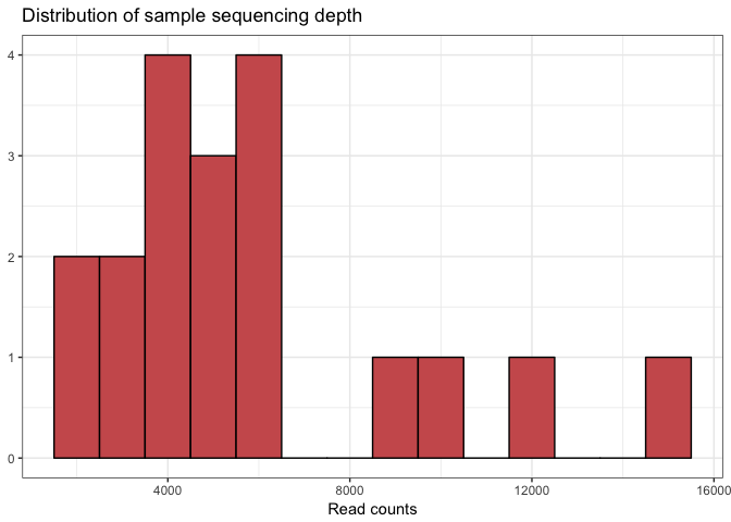
Sample summary

Let’s first look at the number of reads per sample and how that is distributed. We do that by calculating the total number of reads for each of the datasets using the function ** sample_sums**, and then we create a dataframe from the results. Next we feed this dataframe into the **ggplot** function and create a histogram showing the distribution of the read counts.

# Make a data frame with a column for the read counts of each sample
sample_sum_df <- data.frame(sum = sample_sums(mouse_data))

# Histogram of sample read counts
ggplot(sample_sum_df, aes(x = sum)) + 
  geom_histogram(color = "black", fill = "indianred", binwidth = 1000) +
  ggtitle("Distribution of sample sequencing depth") + 
  xlab("Read counts") +
  theme(axis.title.y = element_blank())

But what is the meaning of all these commands inside the ggplot commands? How to understand it, and make use of it? A good place to look for that is found in the ggplot cheat sheet that is found inside the R-studio help menu. And of course google your question and check stackoverflow.com, there you can find lots of solutions on how to use ggplot2.

Any idea what the last line does?
Try adding a label to the y-axis?

The first thing, we want to know are the minimum, average and maximum sample read counts. We use the command ** sample_sums** to calculate that from out data table

# mean, max and min of sample read counts
smin <- min(sample_sums(mouse_data))
smean <- mean(sample_sums(mouse_data))
smax <- max(sample_sums(mouse_data))

# printing the results
cat("The minimum sample read count is:",smin)
cat("The average sample read count is:",smean)
cat("The maximum sample read count is:",smax)

The minimum sample read count is: 2400
The average sample read count is: 5949.895
The maximum sample read count is: 15382

Alpha diversity overview

Now we know the number of reads and we know that the samples show a large variation when it comes to number of reads. Let’s downsample our data, so that we can use it for alpha diversity analysis in R or for any of the other tests we might be interested in. We downsample the data with the command rarefy_even_depth. After that we plot the scaled dataset in a barplot just to check.

# setting the seed to one value in order to created reproducible results
set.seed(1)  

# scaling the mouse data to the smallest samples. Note: rngseed is similar to set.seed
mouse_scaled <- rarefy_even_depth(mouse_data,sample.size=2400, replace=FALSE, rngseed = 1) 

# Make a data frame with a column for the read counts of each sample
plot_bar(mouse_scaled, fill="Class")

With scaled, or beter, rarefied data we can then calculate the alpha diversity for each of the samples and vizualize that in boxplots. We will calculate the same estimators as done in the Mothur MiSeq and add a few more.

# make a vector with the alpha diversity estimators we want to calculate
alpha_meas = c("Observed", "Chao1", "ACE", "Shannon", "Simpson", "InvSimpson")

# plotting the alpha diversity estimators and color by time point
# adding plotting information to object "p"
p <- plot_richness(mouse_scaled, "time", measures=alpha_meas, color="time")

# plot data from "p" as a boxplot with ggplot2
p + geom_boxplot(data=p$data, aes(x=time, color=NULL))

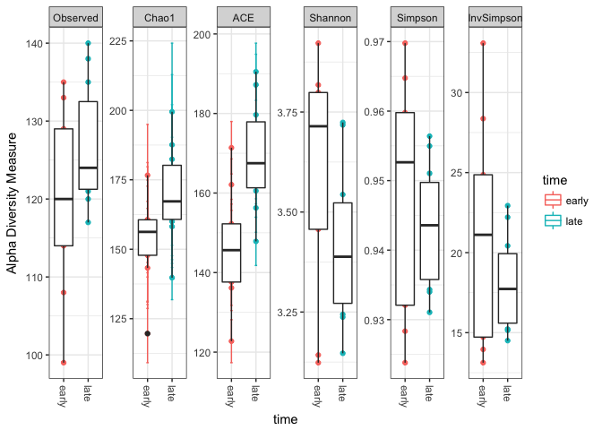
This shows that there is a difference in diversity between the “early” and “late” samples. The number of detected OTUs is for the late samples generaly higher than for the early samples. In addition, it seems that the evenness (Shannon) is lower in the late samples, indicating that the OTU’s are more equal in abundance.

making a rank abundance curve

A final thing to check is to plot a species rank abundance curve. That will give us an idea on the abundance differences between the samples.

# create a vector with the 100 most abundant taxa in the dataset.
topN <- 100
most_abundant_taxa = sort(taxa_sums(mouse_data), TRUE)[1:topN]

#extract most_abundant_taxa from mouse_data
mouse_100_OTUs <- prune_taxa(names(most_abundant_taxa), mouse_data)

# create a dataframe with the counts per otu
mouse_otu_sums <- data.frame(taxa_sums(mouse_100_OTUs))

# use the dataframe to plot the top 100 OTUs in a Rank abundance curve.
ggplot(mouse_otu_sums,aes(x=row.names(mouse_otu_sums), y=taxa_sums.mouse_100_OTUs.)) + 
  geom_bar(stat="identity",colour="black",fill="darkturquoise")  +
  xlab("OTU Rank") + ylab("Number of Sequences per OTU") +
  scale_x_discrete(expand = c(0,0)) + 
  scale_y_continuous(expand = c(0,0)) + theme_classic() +
  ggtitle("Rank Abundance Curve of the Top 100 OTUs") + 
  theme(axis.text.x = element_blank(),
        axis.ticks.x = element_blank())

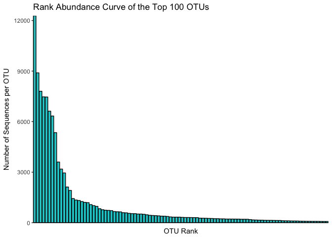
This is a rank-abundance curve, or Whittaker plot, and it mainly shows that some OTU’s are very abundant. The shape of the curve gives us information about the species richness in the entire dataset. What we see here is a typical distribution for microbial communities, with a few OTUs being very abundant and the rest much less abundant. This method is also interesting when comparing samples or treatments, since it can indicate if there is a difference between the communities in how the abundances of the same set of OTUs are distributed.

# extracting read counts from the 100 most abundant OTUs
mouse_early <- prune_taxa(names(most_abundant_taxa), subset_samples(mouse_data, time == "early"))
mouse_late <- prune_taxa(names(most_abundant_taxa), subset_samples(mouse_data, time == "late"))

# making data frames
mouse_early_sums <- data.frame(taxa_sums(mouse_early))
mouse_late_sums <- data.frame(taxa_sums(mouse_late))

# plotting the rank abundance curves as lines, for all samples and early & late samples
plot(sort(mouse_otu_sums$taxa_sums.mouse_100_OTUs., TRUE),ylim=c(1,13000), log="y",
     type="l", cex=2, col="black",
     xlab="OTU rank", ylab="Number of Sequences per OTU (log10)")
lines(sort(mouse_early_sums$taxa_sums.mouse_early., TRUE), type="l", cex=2, col="steelblue")
lines(sort(mouse_late_sums$taxa_sums.mouse_late., TRUE), type="l", cex=2, col="orange2")

# adding a legend to the figure-
legend(70,10000, c("all samples", "early", "late"), col=c("black", "steelblue", "orange2"), pch=19)

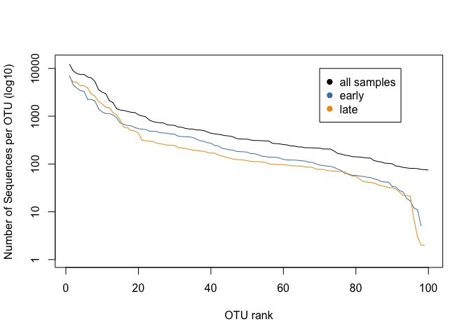
This plot shows us the abundances of the top 100 OTUs for early and late communities, ranked on abundance for each group. * What does that mean? * Can you say something about the abundance of otu0050 in both samples?

Making a dendrogram of the highly abundant OTUs

We have the taxonomic overview from our microbiome samples (final.0.03.taxonomy), and we created earlier a dendrogram from our microbiome data. Togther, we can use those datasets to create a dendrogram with of the top 100 OTU’s, and we can then vizualize them according to their taxonomy.

# plotting the tree
plot_tree(mouse_100_OTUs, color=c("Class"))

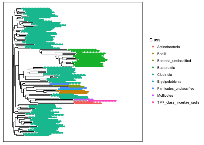
What are the two most abundant phyla in the mouse gut communities ?

This is quite a dense tree, and not easy to reads. Let’s reduce the number of taxa. Instead of using OTUs, based on their abundance ranking, we will select them based on the total number of reads. Say, we pick all OTUs with more than 500 reads in the dataset.

# First remove taxa with less than 500 reads from the mouse_data 
mouse_taxa <- prune_taxa(taxa_sums(mouse_data) >= 500, mouse_data)

# plotting the tree
plot_tree(mouse_taxa, color=c("Class"), shape="time", label.tips = "taxa_names",
          size="abundance", sizebase=10, base.spacing = 0.01, ladderize=TRUE)

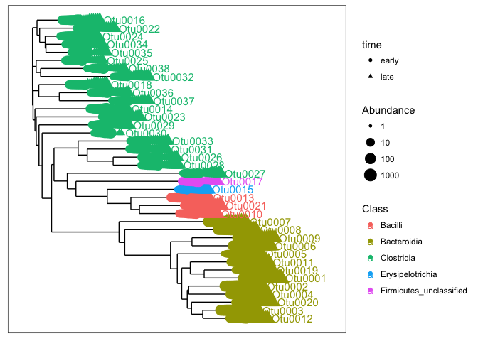
Altough, this is still an intense plot, we now can have an idea of the major taxa in our dataset. These samples are dominated by different classes withing the phyla: Firmicutes and Bacteroidetes. The most abundant taxa (Otu0001 - Otu0009) in our dataset are in the found in the class Bacteroidia. We can also see that some otu’s (e.g. Otu0030) are not present in all samples. The issue with only vizualizing the dominant part of the communities is that we do not get an idea of all the diversity present in our samples. The dendrogram is not really suited for that.

Try plotting a similar dendrogram tree with all the OTUs that have less than 50 reads in the sample. That will show you the diversity of the rare community.

Making a stacked barplot

A better way of showing the taxonomic diversity of our data is to use a barplot. Since we have over 300 OTUs it is difficult to vizualize the abundance of all these “species” in one figure, since there are simply not enough divergent colors that are distinguishable from each other (humans only can seperate about 15 colors in one plot). It is therefor needed to reduce the taxonomic overview. This is however dependent on the taxonomic level that you use.The first thing we need to do is to melt our data into a format that is readable by ggplot2 in order to create a barplot. ggplot likes to have the data in a column based format

# melt to long format (for ggploting) 
# prune out phyla below 1% in each sample
# selecting the taxa at the level: Phylum

mdata_phylum <- mouse_data %>%
  tax_glom(taxrank = "Phylum") %>%                     # agglomerate at phylum level
  transform_sample_counts(function(x) {x/sum(x)} ) %>% # Transform to rel. abundance
  psmelt() %>%                                         # Melt to long format
  filter(Abundance > 0.01) %>%                         # Filter out low abundance taxa
  arrange(Phylum)                                      # Sort data frame alphabetically by phylum

# checking the dataframe that we now created
head(mdata_phylum)

##       OTU Sample  Abundance  group dpw time body_weight  Kingdom
## 1 Otu0059 F3D142 0.01192925 F3D142 142 late       40.18 Bacteria
## 2 Otu0055 F3D143 0.01750000 F3D143 143 late       39.16 Bacteria
## 3 Otu0055 F3D148 0.01371308 F3D148 148 late       40.74 Bacteria
## 4 Otu0055 F3D142 0.01234060 F3D142 142 late       40.18 Bacteria
## 5 Otu0055 F3D141 0.01083424 F3D141 141 late       39.37 Bacteria
## 6 Otu0001 F3D145 0.78530155 F3D145 145 late       40.33 Bacteria
##                  Phylum
## 1        Actinobacteria
## 2 Bacteria_unclassified
## 3 Bacteria_unclassified
## 4 Bacteria_unclassified
## 5 Bacteria_unclassified
## 6         Bacteroidetes

The table shows that we have the samples randomly troughout the dataset, but we have the phylum names alphabetically sorted. That makes the barplot phylum ordering nicer too read.

There is five taxa in this dataset at the phylum level. So we only need five colors for displaying them.

phylum_colors <- c("steelblue", "red", "orange","magenta", "maroon")

Using these five colors we can now plot the bargraph.

ggplot(mdata_phylum, aes(x = Sample, y = Abundance, fill = Phylum)) + 
  #facet_grid(time~.) +
  geom_bar(stat = "identity") +
  scale_fill_manual(values = phylum_colors) +
  scale_x_discrete(
    breaks = map$group,
    labels = map$group, 
    drop = FALSE
  )  +
  # Remove x axis title, and rotate sample lables
  theme(axis.title.x = element_blank(),
        axis.text.x=element_text(angle=90,hjust=1,vjust=0.5)) + 
  
  # additional stuff
  guides(fill = guide_legend(reverse = TRUE, keywidth = 1, keyheight = 1)) +  # modifying the legend
  ylab("Relative Abundance (Phyla > 1%) \n") +
  ggtitle("Phylum Composition of Mothur MiSeq SOP data per individual") 

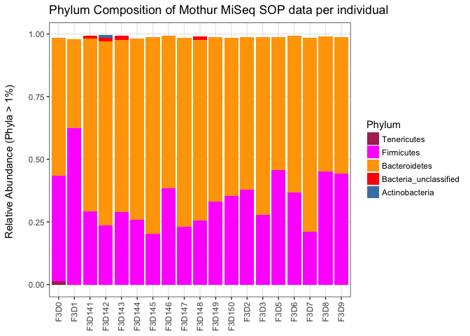
The first thing I notice when looking at the x-axis is that the samples are not ordered. We can do that by using the following addition to first list of the commands:

replace "Sample" with "reorder(Sample, dpw)".

After running the ggplot command with the modification, we see that the samples are ordered correctly.

Notice how the bars do not fill up to 1. What is the meaning of that? What part of the community is missing?

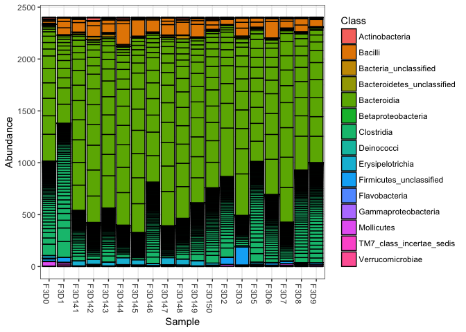
a stacked barplot for the class level

Let’s repeat the barplotwith a slightly different taxonomic level. We now pick the level class and try to identify which taxa make up more than 1 % of the reads.

# melt to long format (for ggploting) 
# prune out phyla below 1% in each sample
# selecting the taxa at the level: Phylum

mdata_class <- mouse_data %>%
  tax_glom(taxrank = "Class") %>%                     # agglomerate at phylum level
  transform_sample_counts(function(x) {x/sum(x)} ) %>% # Transform to rel. abundance
  psmelt() %>%                                         # Melt to long format
  filter(Abundance > 0.01) %>%                         # Filter out low abundance taxa
  arrange(Class)                                      # Sort data frame alphabetically by phylum

str(mdata_class)

## 'data.frame':    77 obs. of  10 variables:
##  $ OTU        : chr  "Otu0059" "Otu0010" "Otu0010" "Otu0010" ...
##  $ Sample     : chr  "F3D142" "F3D144" "F3D3" "F3D6" ...
##  $ Abundance  : num  0.0119 0.0949 0.0765 0.0747 0.0734 ...
##  $ group      : Factor w/ 19 levels "F3D0","F3D1",..: 4 6 14 16 11 7 9 2 4 18 ...
##  $ dpw        : int  142 144 3 6 149 145 147 1 142 8 ...
##  $ time       : chr  "late" "late" "early" "early" ...
##  $ body_weight: num  40.2 41.6 15.5 20.5 40.6 ...
##  $ Kingdom    : Factor w/ 1 level "Bacteria": 1 1 1 1 1 1 1 1 1 1 ...
##  $ Phylum     : Factor w/ 9 levels "Actinobacteria",..: 1 5 5 5 5 5 5 5 5 5 ...
##  $ Class      : Factor w/ 15 levels "Actinobacteria",..: 1 2 2 2 2 2 2 2 2 2 ...

There is fifteen taxa in this dataset at the class level. So we need fifteen colors for vizualizing them. I have used a set of colors that are written in hexidecimal code. An overview of colors available in R can be found online. This is a nice cheatsheet, a pdf with colornames, and the website Rcolorbrewer to pick colors readable for colorblind people, or for different kinds of data.

class_colors <- c("#CBD588", "#5F7FC7", "orange","#DA5724", "#508578", "#CD9BCD",
  "#AD6F3B", "#673770","#D14285", "#652926", "#C84248", 
  "#8569D5", "#5E738F","#D1A33D", "#8A7C64", "#599861")

Then we plot the class level taxa that make up at least 1 % of the data.

ggplot(mdata_class, aes(x = reorder(Sample, dpw), y = Abundance, fill = Class)) + 
  #facet_grid(time~.) +
  geom_bar(stat = "identity") +
  scale_fill_manual(values = class_colors) +
  scale_x_discrete(
    breaks = map$group,
    labels = map$group, 
    drop = FALSE
  )  +
  # Remove x axis title, and rotate sample labels
  theme(axis.title.x = element_blank(),
        axis.text.x=element_text(angle=90,hjust=1,vjust=0.5)) + 
  
  # additional stuff
  guides(fill = guide_legend(reverse = TRUE, keywidth = 1, keyheight = 1)) +
  ylab("Relative Abundance (Class > 1%) \n") +
  ggtitle("Class Composition of Mothur MiSeq SOP data per individual") 

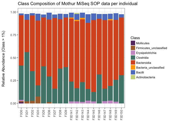
This gives us more insight in the diversity found in our samples. It is suggested from this that there is a decline in the relative abundances of the Clostridia OTUs. That could be possible, but one should not be too quick in writting that down.

Why are relative abundances between samples difficult to interpret?
What is lost from the data when you use relative abundances?

Relative abundances are one way of standardizing samples to be more equal. There is many methods that can be used, such as log transformations (to make data more normally distributed), normalizations around zero (z-score), resampling to either the lowest, median or highest sample abundance, to name a few. Most methods comes with their own pitfalls, and more importantly statistical method have their requirements as well. Remember that a T-test can only be used for normally distributed data. With many methods in for exploring microbiome data it can make a difference what kind of standardization / normalisation you use, so it is good to read the manual before trying out new statistical test on your own data.

Unconstrained ordinations

On of the best ways to explore microbiome data is with ordination techniques / multivariate analysis techniques. The first step is to do unconstrained ordinations. Here we will try our Principle coordinate Analysis (PCoA). But before we can plot our data in an ordination, we need to make it suitable by subsampling or rarefying the data. Note that the authors of phyloseq do not like rarefying, but rather recommend the technique provided with the RNA-seq tool Deseq2. Nonetheless, they do provide a method to rarefy your data. We will take a look at Deseq2 later on in this tutorial.

#### unconstrained ordinations
# rarefying reads to even depth (Note that this is not recommended by the phyloseq authors)
mouse_scaled <- rarefy_even_depth(mouse_data, sample.size = 2400, replace = FALSE, rngseed = 1)

Next we run the ordinate command with the PCoA method to generate a an object containing the PCoA results.

# Ordinate using Principal Coordinate analysis
mouse_pcoa <- ordinate(
  physeq = mouse_scaled, 
  method = "PCoA", 
  distance = "bray"
)

# Or write in short format
mouse_pcoa <- ordinate(mouse_scaled, "PCoA", "bray")

The first thing to do after run an ordination is to make a scree plot. A scree plot gives us an overview of the variance explained by the axis in the ordination and is an important tool to understand the validity of the ordination.

# checking the ordination by making a scree plot
plot_ordination(
  physeq = mouse_scaled,
  ordination = mouse_pcoa,
  type="scree")

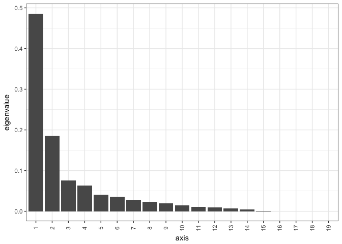
This shows us that the first axis explains almost 50 % of the data, and the second axis explains another 18 %. Now we know that we only need to focus on the first two axis to explain almost 70% of the variation in the dataset.

How many axis are there in the dataset?

# Plot 
plot_ordination(
  physeq = mouse_scaled,
  ordination = mouse_pcoa,
  axes=c(1,2),   # this selects which axes to plot from the ordination
  color = "time",
  shape = "time",
  label = "group", # not really needed but can be useful for exploration
  title = "PCoA of mouse gut bacterial Communities"
) + 
  scale_color_manual(values = c("steelblue", "orange")
  ) +
  geom_point(aes(color = time), alpha = 0.7, size = 4) +
  geom_point(colour = "grey90", size = 1.5)+
  geom_text(label= "group", size=2)

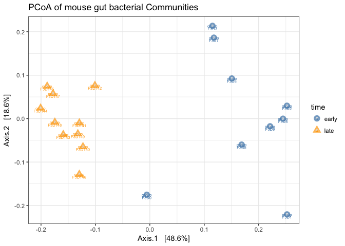
Note that by using color and shapes we can represent multiple layers of information about our data on this ordination plot.

Try changing the axis that you plot and observe what that does with the ordination.
Add to the plot_ordination command the ggplot function: “geom_line()”. What happens and is this usefull?

With this ordination we can clearly see a seperation between the time points based on the OTU community composition.

Unconstrained ordination of OTUs

A method like PCoA is not able to directly show the clustering of OTUs and how they are different from each other for each of the datasets. That is something we are often not interested in, but it could be nice to see how to do that. We can do that using Non-Metric Multidimensional Scaling (NMDS). NMDS is an ordination method that tries to reduce the amount of residual distances (not shown) in the first two or three axes. It tries to coverge to a stable solution. After running the following command you can see that the script produces the testing. It looks for the ordination with the lowest stress. It is therefor important to report the stress value and it should be lower than 0.2. Anything above is not to be trusted.

# running ndms on mouse scaled data
mouse_otu_nmds <- ordinate(mouse_scaled, "NMDS", "bray")

## Square root transformation
## Wisconsin double standardization
## Run 0 stress 0.1106345 
## Run 1 stress 0.1245127 
## Run 2 stress 0.1392333 
## Run 3 stress 0.1386702 
## Run 4 stress 0.1278278 
## Run 5 stress 0.1393336 
## Run 6 stress 0.1109244 
## ... Procrustes: rmse 0.01584889  max resid 0.05597805 
## Run 7 stress 0.1109242 
## ... Procrustes: rmse 0.01589432  max resid 0.05616951 
## Run 8 stress 0.1386701 
## Run 9 stress 0.1329519 
## Run 10 stress 0.1468084 
## Run 11 stress 0.1270008 
## Run 12 stress 0.1490718 
## Run 13 stress 0.1109242 
## ... Procrustes: rmse 0.01586424  max resid 0.0560563 
## Run 14 stress 0.1278268 
## Run 15 stress 0.1420973 
## Run 16 stress 0.1322715 
## Run 17 stress 0.1488085 
## Run 18 stress 0.1386701 
## Run 19 stress 0.1476136 
## Run 20 stress 0.1316211 
## *** No convergence -- monoMDS stopping criteria:
##     20: stress ratio > sratmax

# printing stress level
cat("stress is:", mouse_otu_nmds$stress)

## stress is: 0.1106345

#ordination plot using the otus, and color by Phylum
plot_ordination(mouse_scaled, mouse_otu_nmds, type="taxa", color="Phylum", title="NMDS ordination - OTUs")

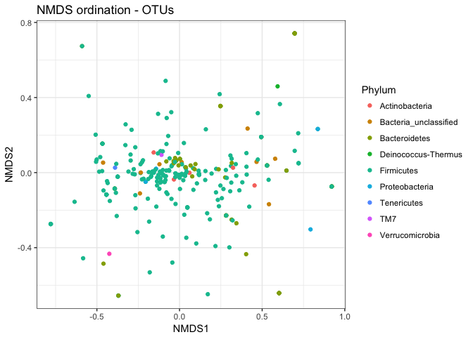
This ordination is a bit hard to read since a lot of the taxa are present and points are overlapping. Let’s add the facet function within the ggplot2 package to this ordination, to split the ordination in to ordinations per taxon.

plot_ordination(mouse_scaled, mouse_otu_nmds, type="taxa", color="Phylum", title="taxa") +
  facet_wrap(~Phylum, 3)

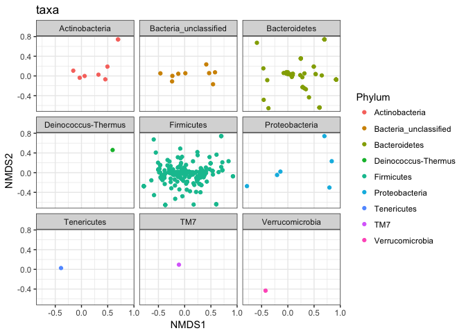
This is shows that some OTUs in the various taxa are possbly reponsible for the variation between the taxa.

Let’s run the plot_ordination command on the samples instead of the OTUs. We can use the same ordination object as above.

plot_ordination(mouse_scaled, mouse_otu_nmds,
                type="samples",
                color="time",
                shape="time",
                title="NDMS ordination - Samples",
                label = "group" # not really needed but can be useful for exploration
) +
  scale_color_manual(values = c("steelblue", "orange2")
  ) +
  geom_point(aes(color = time), alpha = 0.7, size = 4) +
  geom_point(colour = "grey90", size = 1.5)

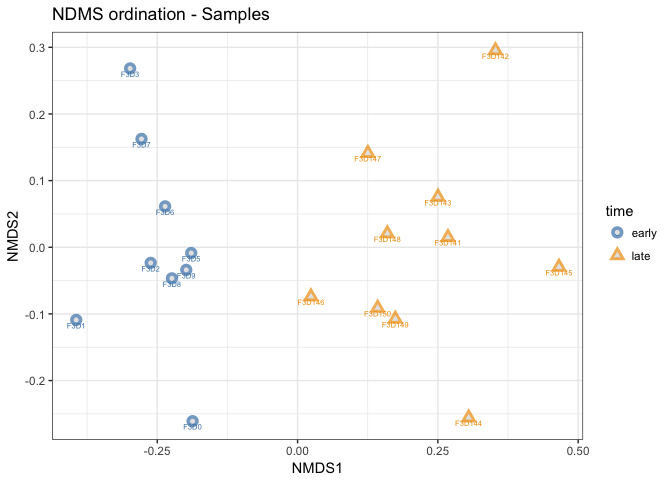
How is this plot different from the PCoA we created before?

Simper analysis

In our data example here we only have time as a factor mainly reponsible for the differences. But in the case of many factors (like environmental chemistry data), you might want to identify which factors are reponsible for the differences between the samples. One way to test this is with a procedure that breaks down similarity percentages (SIMPER). The vegan package comes with the simper command. It uses permutation and uses a bray-curtis to calculate the distances between the samples. Our job is to provide simper with a OTU table and factor that we want to test from out metadata table.

## Simper analysis, extract abundance matrix from a phyloseq object
mouse_OTUs = as(otu_table(mouse_scaled), "matrix")

# transpose so we have the OTUs as columns
if(taxa_are_rows(mouse_scaled)){mouse_OTUs <- t(mouse_OTUs)}

# Coerce the object to a data.frame
mouse_OTUs_scaled = as.data.frame(mouse_OTUs)

# running the simper analysis on the dataframe and the variable of interest "time"
mouse_simper <- simper(mouse_OTUs_scaled, map$time, permutations = 100)

# printing the top OTUs
print(mouse_simper)

## cumulative contributions of most influential species:
## 
## $early_late
##   Otu0005   Otu0004   Otu0001   Otu0007   Otu0010   Otu0008   Otu0006 
## 0.1154843 0.1743518 0.2257156 0.2733079 0.3145751 0.3534291 0.3906387 
##   Otu0002   Otu0013   Otu0017   Otu0014   Otu0015   Otu0009   Otu0003 
## 0.4185430 0.4422606 0.4627904 0.4829891 0.5031148 0.5221237 0.5407453 
##   Otu0016   Otu0019   Otu0012   Otu0011   Otu0030   Otu0018   Otu0026 
## 0.5588899 0.5761926 0.5933438 0.6074644 0.6196150 0.6315524 0.6431811 
##   Otu0022   Otu0025   Otu0029   Otu0035   Otu0021   Otu0043 
## 0.6544225 0.6650578 0.6750926 0.6844876 0.6935010 0.7022674

# for more details on the simper output use "summary"
# summary(mouse_simper)

This table shows us the OTUs that make up 70% of the differences between the groups, and how much they contribute to the observed sample clustering. The simper results are not so easy to interpret. The summary function shows a little more info and indicates which species show a different abundance between the treatments or groups. For instance otu00001, with the largest abundance in this dataset is not significantly different in abundance with this simper analysis.

What is the contribution of Otu0021 and Otu0043?

Altough Simper can identify differentialy abundant taxa, other tests like Metastats (see mothur) or Deseq2 are better methods to identify differentialy abundandant taxa. We will try out Deseq 2 later, but first more ordinations.

Unifrac analysis of community composition

Both NMDS and PCoA are often used to display the results from a Unifrac analysis. Unifrac is a method that use a phylogenetic tree to identify if communities are significantly different from each other.

Here we will run Unifrac on our microbial community data that contains a phylogenetic tree of the OTUs. Note that you can also do this within Mothur or QIIME. Furthermore, note that we use the scaled data for this since the unifrac method is sensitive to sampling effort. It is thus needed to rarefy the samples or any other normalization technique. For more info on unifrac see the publication from Luzopone et al., 2011 and references in there.

# creating a distance matrix using unweigthed unifrac distances
mouse_Unifrac_NoW <- UniFrac(mouse_scaled, weighted = FALSE)

# calculation of the NMDS using the unweigthed unifract distances
mouse_unifrac_NoW_nmds <- ordinate(mouse_scaled, "NMDS", mouse_Unifrac_NoW)

## Run 0 stress 0.1197003 
## Run 1 stress 0.1531076 
## Run 2 stress 0.126869 
## Run 3 stress 0.1197003 
## ... New best solution
## ... Procrustes: rmse 5.112737e-06  max resid 1.454828e-05 
## ... Similar to previous best
## Run 4 stress 0.1418309 
## Run 5 stress 0.1197003 
## ... New best solution
## ... Procrustes: rmse 1.042145e-06  max resid 1.686025e-06 
## ... Similar to previous best
## Run 6 stress 0.1299261 
## Run 7 stress 0.1632334 
## Run 8 stress 0.1342403 
## Run 9 stress 0.1418306 
## Run 10 stress 0.14115 
## Run 11 stress 0.1387266 
## Run 12 stress 0.1286217 
## Run 13 stress 0.1378198 
## Run 14 stress 0.1285092 
## Run 15 stress 0.1197003 
## ... Procrustes: rmse 3.37225e-06  max resid 1.013216e-05 
## ... Similar to previous best
## Run 16 stress 0.126869 
## Run 17 stress 0.139139 
## Run 18 stress 0.1299261 
## Run 19 stress 0.139097 
## Run 20 stress 0.1197003 
## ... Procrustes: rmse 1.427674e-06  max resid 3.841933e-06 
## ... Similar to previous best
## *** Solution reached

cat("stress is:", mouse_unifrac_NoW_nmds$stress)

## stress is: 0.1197003

So the stress is below 0.2, but it is not perfect. We would tather have it below 0.1, but this is what we have.

# Plotting the ordination, 
p1 <- plot_ordination(mouse_scaled, mouse_unifrac_NoW_nmds,
                type="samples",
                color="time",
                shape="time",
                title="NDMS unifrac Unweighted",
                label = "group" # not really needed but can be useful for exploration
) +
  scale_color_manual(values = c("steelblue", "orange2")
  ) +
  geom_point(aes(color = time), alpha = 0.7, size = 4) +
  geom_point(colour = "grey90", size = 1.5)

# plotting object p1
print(p1)

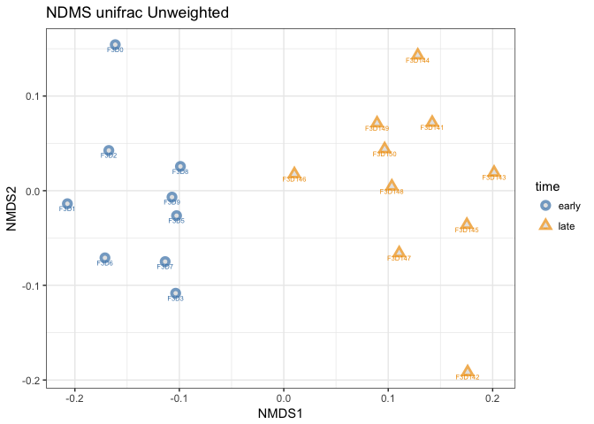
This is not much different from the NDMS using bray-curtis distances. Note that I now assigned the output of plot_ordination to a object called p1. I did that because I want to compare how weighted and unweighted unifrac affects the ordination. Let’s try that.

## create weighted unifrac ordination and compare with unweighted
mouse_Unifrac_W <- UniFrac(mouse_scaled, weighted = TRUE, 
                             parallel = TRUE)
# calculation of the NMDS using the unweigthed unifract distances
mouse_unifrac_W_nmds <- ordinate(mouse_scaled, "NMDS", mouse_Unifrac_W)

## Run 0 stress 0.05420305 
## Run 1 stress 0.1042102 
## Run 2 stress 0.05420239 
## ... New best solution
## ... Procrustes: rmse 0.0002111106  max resid 0.0006913747 
## ... Similar to previous best
## Run 3 stress 0.05420256 
## ... Procrustes: rmse 0.0003471439  max resid 0.001155513 
## ... Similar to previous best
## Run 4 stress 0.1041606 
## Run 5 stress 0.05420305 
## ... Procrustes: rmse 0.0004744802  max resid 0.001577066 
## ... Similar to previous best
## Run 6 stress 0.05420266 
## ... Procrustes: rmse 0.0003745221  max resid 0.001247995 
## ... Similar to previous best
## Run 7 stress 0.1072737 
## Run 8 stress 0.1042107 
## Run 9 stress 0.05420232 
## ... New best solution
## ... Procrustes: rmse 0.0001442819  max resid 0.0004792946 
## ... Similar to previous best
## Run 10 stress 0.09914907 
## Run 11 stress 0.1043675 
## Run 12 stress 0.3259743 
## Run 13 stress 0.0542024 
## ... Procrustes: rmse 0.0001235274  max resid 0.0004092409 
## ... Similar to previous best
## Run 14 stress 0.05420274 
## ... Procrustes: rmse 0.0001953769  max resid 0.0006451767 
## ... Similar to previous best
## Run 15 stress 0.05420256 
## ... Procrustes: rmse 0.0001699845  max resid 0.0005550827 
## ... Similar to previous best
## Run 16 stress 0.104157 
## Run 17 stress 0.1042622 
## Run 18 stress 0.05420233 
## ... Procrustes: rmse 7.623009e-05  max resid 0.0002439109 
## ... Similar to previous best
## Run 19 stress 0.05420233 
## ... Procrustes: rmse 6.809302e-05  max resid 0.0002194473 
## ... Similar to previous best
## Run 20 stress 0.0542025 
## ... Procrustes: rmse 0.0001841636  max resid 0.0006100906 
## ... Similar to previous best
## *** Solution reached

cat("stress is:", mouse_unifrac_W_nmds$stress)

## stress is: 0.05420232

# Plotting the ordination
p2 <- plot_ordination(mouse_scaled, mouse_unifrac_W_nmds,
                      type="samples",
                      color="time",
                      shape="time",
                      title="NDMS unifrac Weighted",
                      label = "group" # not really needed but can be useful for exploration
) +
  scale_color_manual(values = c("steelblue", "orange2")
  ) +
  geom_point(aes(color = time), alpha = 0.7, size = 4) +
  geom_point(colour = "grey90", size = 1.5)

# combine plots p1 and p2 into one figure with the plot_grid command (cowplot)
plot_grid(p1, p2, labels = c("P1", "P2"), ncol = , nrow = 1, rel_widths=c(2,2))

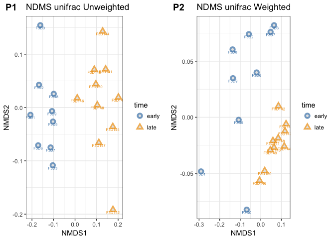
The side-by-side plotting of the ordinations shows us that using weighting makes quite a difference.

Can you spot the differences between these two plots?
Which ordination has the better stress level?
What does that tell us about both communities?

Significance testing of the Unifrac results

Altough we can see clear seperation in an ordination of the samples based on time, it is good to test this in a more appropriate way. There are several methods we can use, such as : Analysis of Similarities (ANOSIM). This is a permutational non-parametric test of significance of the sample-grouping against a null-hypothesis. The default number of permutations is 999. The method identifies of the between groups difference is larger than the within groups difference.

## testing of significance for the unifrac ordinations using ANOSIM
# create vector with time point labels for each samples
mouse_time <- get_variable(mouse_scaled, "time")

# run Anosim on a unweighted Unifrac distance matrix of the mouse_scaled OTU table, with the factor time
mouse_anosim_UFuW <- anosim(distance(mouse_scaled, "unifrac", weighted=FALSE), mouse_time)

# run Anosim on a Weighted Unifrac distance matrix of the mouse_scaled OTU table, with the factor time
mouse_anosim_UFW <- anosim(distance(mouse_scaled, "unifrac", weighted=TRUE), mouse_time)

#plot results
print(mouse_anosim_UFuW)

## 
## Call:
## anosim(dat = distance(mouse_scaled, "unifrac", weighted = FALSE),      grouping = mouse_time) 
## Dissimilarity: 
## 
## ANOSIM statistic R: 0.851 
##       Significance: 0.001 
## 
## Permutation: free
## Number of permutations: 999

print(mouse_anosim_UFW)

## 
## Call:
## anosim(dat = distance(mouse_scaled, "unifrac", weighted = TRUE),      grouping = mouse_time) 
## Dissimilarity: 
## 
## ANOSIM statistic R:   0.6 
##       Significance: 0.001 
## 
## Permutation: free
## Number of permutations: 999

# when interested in only if the grouping is significant, do
# mouse_anosim$signif

As expected the grouping is highly significant and it is so for both the weighted and the unweighted unifrac results. It indicates that there is a significant differences between the early and late mouse gut communities.

The dataset created by the anosim can also be queried with the R functions: summary() and plot().

explore the anomsim dataset with both functions. What is actually tested here? (See also the helpfile for anosim)

Another method that can be used in Multivariate analysis of variance(MANOVA), and is similar to a univariate ANOVA test. MANOVA is a parametric test, and that is a problem for microbiome datasets, which often violate the assumptions of MANOVA. A non-parametric test is available and it called PERMANOVA. This test is present in the vegan package as the command: adonis. Let’s explore this using the weighted unifrac distance matrix.

# run a permanova test with adonis.
set.seed(1)

# Calculate bray curtis distance matrix
mouse_unifrac_W <- phyloseq::distance(mouse_scaled, method = "unifrac", weighted=TRUE)

# make a data frame from the scaled sample_data
sampledf <- data.frame(sample_data(mouse_scaled))

# Adonis test
adonis(mouse_unifrac_W ~ time, data = sampledf)

## 
## Call:
## adonis(formula = mouse_unifrac_W ~ time, data = sampledf) 
## 
## Permutation: free
## Number of permutations: 999
## 
## Terms added sequentially (first to last)
## 
##           Df SumsOfSqs  MeanSqs F.Model      R2 Pr(>F)    
## time       1   0.14052 0.140523  10.166 0.37421  0.001 ***
## Residuals 17   0.23499 0.013823         0.62579           
## Total     18   0.37552                  1.00000           
## ---
## Signif. codes:  0 '***' 0.001 '**' 0.01 '*' 0.05 '.' 0.1 ' ' 1

With this analysis we can conclude that there is a significant differences between the groups of our dataset and we reject the null hypothesis. However, we do have an indication from the alpha diversity that the evenness between our groups is different. That could be the cause of the difference in communities here, so before fully excepting the adonis test we need to run a test to check for the homogeneity of variances when comparing these groups. We use the vegan command betadisper, which is a multivariate test for homogeneity of group dispersions (variances). In addition, do we run a permutational test to get a test-statistic.

# test of Homegeneity of dispersion
beta <- betadisper(mouse_unifrac_W, sampledf$time)

# run a permutation test to get a statistic and a significance score
permutest(beta)

## 
## Permutation test for homogeneity of multivariate dispersions
## Permutation: free
## Number of permutations: 999
## 
## Response: Distances
##           Df   Sum Sq   Mean Sq      F N.Perm Pr(>F)    
## Groups     1 0.017141 0.0171411 10.937    999  0.001 ***
## Residuals 17 0.026645 0.0015673                         
## ---
## Signif. codes:  0 '***' 0.001 '**' 0.01 '*' 0.05 '.' 0.1 ' ' 1

The betadisper test is significant (p < 0.01), so we have to accept that our datasets do not have the same variances. So we should be cautious in interpreting our weighted unifrac ordination. We can not simply say that the communities consist of different OTUs. Among the two groups there is a difference in the abundances between the OTUs. Or better the evenness is different between these two groups.

What do you expect when you test the unweighted unifrac results with adonis and betadispers? Is there still a significant difference? Why is that?

Constrained ordination

Constrained ordinations are usefull to explore the relationship of environmental or host associated parameters with the diversity found in our samples. In this example we do not really have such data, but we can still use time to constrain at least one axis of our ordinations, and then plot our samples accordingly. We do not use NMDS or PCoA, but we use correspondance analysis and method that uses a Chi-square transformed data matrix that is subjected to linear regression of contraining variables.

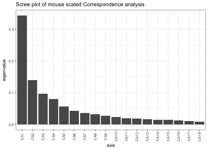
# constrained ordination test using Correspondence Analysis (CA)

mouse_CA <- ordinate(mouse_scaled, "CCA")

# check ordination with a scree plot
plot_scree(mouse_CA, "Scree plot of mouse scaled Correspondence analysis")

(p1_CA <- plot_ordination(mouse_scaled, mouse_CA, "samples",
                          color="time",shape="time", label="body_weight") +
    scale_color_manual(values = c("steelblue", "orange2")) +
    geom_point(aes(color = time), alpha = 0.4, size = 4))

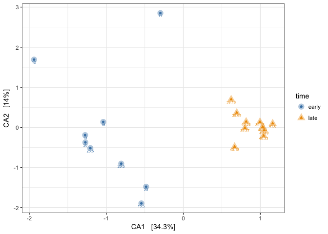
Observed how the samples are arranged. We added the tiny FAKE body_weight values for extra information just to observe how they are distributed, over these gut communities that are from a time series.

# Now doing a constrained Correspondence Analysis (CCA), using time
mouse_CCA <- ordinate(mouse_scaled, formula = mouse_scaled ~ time + body_weight, "CCA")

# check ordination with a scree plot
plot_scree(mouse_CCA, "Scree plot of mouse scaled Constrained Correspondence analysis")

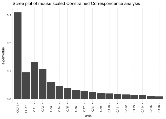
What axes are indicated in this scree plot. What happens if you remove body_weight from the ordinate command?

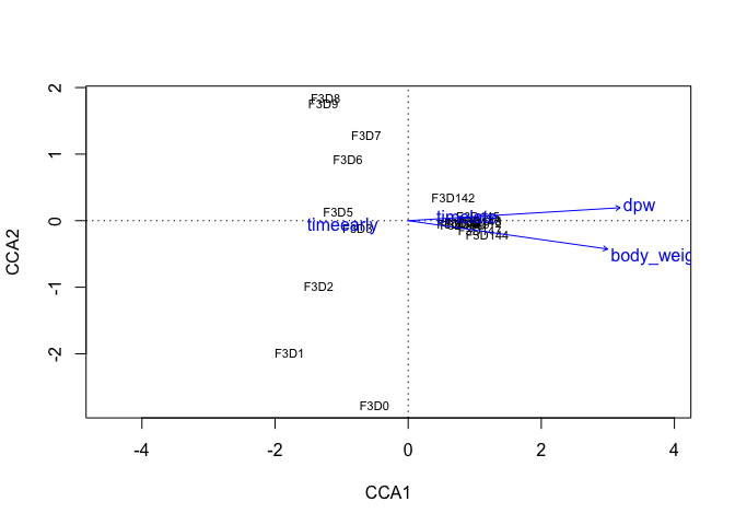
# CCA plot
CCA_plot <- plot_ordination(mouse_scaled, mouse_CCA, type="samples", color="time", shape="time", label="body_weight") + 
  scale_color_manual(values = c("steelblue", "orange2")
  ) +
  geom_point(aes(color = time), alpha = 0.4, size = 4)

# Now add the environmental variables as arrows into a matrix
arrowmat <- vegan::scores(mouse_CCA, display = "bp")

# transform matrix into a dataframe, and add labels
arrowdf <- data.frame(labels = rownames(arrowmat), arrowmat)


# Define the arrow aesthetic mapping
arrow_map <- aes(xend = CCA1, 
                 yend = CCA2, 
                 x = 0, 
                 y = 0,
                 shape= NULL,
                 color= NULL,
                 label=labels)

label_map <- aes(x = 1.2 * CCA1, 
                 y = 1.2 * CCA2,
                 shape= NULL,
                 color= NULL,
                 label=labels)

arrowhead = arrow(length = unit(0.02, "npc"))

# Make a new graphic
CCA_plot + 
  geom_segment(
    mapping = arrow_map, 
    size = .5, 
    data = arrowdf, 
    color = "gray", 
    arrow = arrowhead
  ) + 
  geom_text(
    mapping = label_map, 
    size = 4,  
    data = arrowdf, 
    show.legend = FALSE
  )

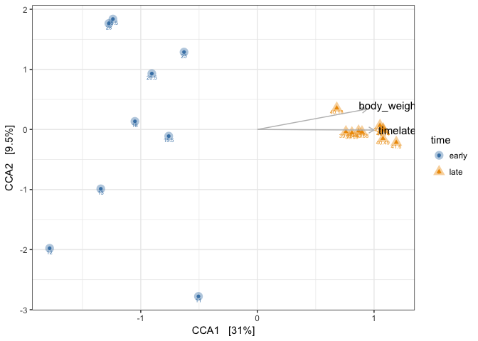
Body_weight of mouse pups should be increasing over time, while the weight of the adults should not increase. In our fake body_weights, we had an unnatural increase in the adults body weight after day 145. What you see here is how the samples are now placed in the ordination, with respect to their time point and their bodyweight. If we had more variables we could have fitted those on top of this constrained ordination and observed how they correlate with the constrained factors. This is method is usefull for identifying factor, that explain the variation in your microbiome. This example is just an introduction, and better examples can be found in the source listed at the top of this tutorial.

Above with did CCA with two constrain axes, but that is not always needed. You can very well do an ordination with only one axes constrained. For the above example, you could only decide to constrain on “time”. The results will be that in the script you need to replace CCA2 with CA1 and that vizualize it.

Last thing to do is test for significance with a permutational anova test.

# permutational anova test on constrained axes
anova(mouse_CCA)

## Permutation test for cca under reduced model
## Permutation: free
## Number of permutations: 999
## 
## Model: cca(formula = OTU ~ time + body_weight, data = data)
##          Df ChiSquare      F Pr(>F)    
## Model     2   0.23392 5.4516  0.001 ***
## Residual 16   0.34327                  
## ---
## Signif. codes:  0 '***' 0.001 '**' 0.01 '*' 0.05 '.' 0.1 ' ' 1

When working with a lot of variables it is good to first explore which variables show auto-correlation and only keep those that are dominant. After that you can use the vegan command envfit to check which variables show a significant correlation with the ordination that you give it. for more on that I recommend going through the vegan tutorial (PDF). The results from envfit can be plotted directly on a “normal” R-plot. Here is a short example using our own data.

# run envit for testing
ef <- envfit(mouse_CA, map, permutations = 999)

# plot the ordination data directly using plot
plot(mouse_CCA, display="sites" )

# overly plot with fitted variables
plot(ef, p.max= 0.001)

It is not so pretty as the ggplot2 based graphics, but for exploration, this is usefull. Note that one of the vectors is the label of the sample data: “dpw”.

try plotting the ordination with “species” instead of “sites”.

Identification of differential abundant OTUs

To be added.

heatmap of OTUs

To be added

BioinfTraining

Repository for bioinformatics training at the Norwegian Veterinary Institute